Listening
to the Cosmos: How the Fourier Transform Finds a Pulsar 11,750
Light-Years Away
In 1932, an engineer trying to fix telephone static accidentally
discovered that the Milky Way was broadcasting on radio. What he set in
motion — a sequence of tools, algorithms, and acts of patience —
eventually produced the first photograph of a black hole. This is the
story of what listening to the universe requires.
The engineer and the noise
In 1932, a twenty-six-year-old engineer at Bell Telephone
Laboratories named Karl Jansky was given a straightforward industrial
assignment: identify the sources of static interfering with
transatlantic radio telephone links. The project had a practical
deadline and a practical budget. Jansky built what the assignment
required — a rotating directional antenna, four hundred kilograms of
steel tubing mounted on wheels salvaged from a Model T Ford, the whole
structure completing one full rotation every twenty minutes. He pointed
it at the sky and began listening.
He found what he expected — atmospheric noise, static from
thunderstorms, local interference — and then, after months of systematic
observation, something he did not expect: a persistent hiss that rotated
with the stellar background, not with the Sun. By the process of
eliminating thunderstorms, aircraft, nearby industry, and every artefact
of his own equipment as possible explanations, Jansky arrived at the
only conclusion left. The Milky Way was emitting radio waves at 20.5
MHz. He published this in 1933 in the Proceedings of the Institute
of Radio Engineers — a journal read by telecommunications
engineers, not by astronomers.
The astronomical community largely ignored the paper for nearly a
decade.
Bell Labs, its static problem solved, reassigned Jansky to other
projects. He moved on to vacuum tube amplifier research, then wartime
work. He never returned to radio astronomy. The rotating antenna that
had, incidentally, discovered an entire branch of science was dismantled
for wartime scrap metal. Karl Jansky died in 1950 at forty-four, of a
complication of the hypertension that had troubled him for years. The
unit of radio flux density — the Jansky, 10⁻²⁶ watts per square metre
per hertz — was named in his honour, posthumously, in 1973.
This is, as the engineering guide that underlies this post puts it,
“characteristically, how a new field begins: an engineer notices that
the sky is making noise, reports it in the wrong journal, and the
universe waits patiently for everyone to catch up.”
A clock nobody built
In August 1982, a team at Arecibo Observatory in Puerto Rico — Donald
Backer, Shrinivas Kulkarni, Carl Heiles, Michael Davis, and Woodruff
Sullivan — discovered a radio source in Vulpecula pulsing at 1.5578
milliseconds per period. The previous record for pulsar spin had been
6.1 milliseconds. The new record beat it by a factor of four.
The source was a neutron star.
A neutron star is what remains after a massive star exhausts its
nuclear fuel and its iron core collapses. The collapse happens in the
fraction of a second it takes for a star to decide it is no longer
viable as a star. Roughly 1.4 solar masses compresses into a sphere
approximately twenty kilometres across — smaller than a city.
Conservation of angular momentum does what it always does when a
rotating object shrinks dramatically. PSR B1937+21, the Vulpecula
pulsar, rotates 641.9 times per second. Its equatorial surface moves at
approximately 14% of the speed of light. This is not a metaphor or an
order-of-magnitude estimate; it is what fifty years of precise timing
data say.
The pulsar emits a narrow beam of radio waves with every rotation.
Every 1.5578 milliseconds, that beam sweeps past Earth, producing a
brief radio flash — a pulse arriving 641.9 times per second, from a
source 11,750 light-years away, each pulse having departed approximately
11,750 years before it arrived.
The physical parameters, as tabulated in the Australia Telescope
National Facility Pulsar Catalogue:
| Parameter | Value | Physical meaning |
|---|---|---|
| Spin period P | 1.5578064688 ms | Time per rotation |
| Spin frequency f_spin | 641.9 Hz | Rotations per second |
| Period derivative Ṗ | 1.051 × 10⁻¹⁹ s/s | Rate at which period lengthens |
| Dispersion measure DM | 71.025 pc cm⁻³ | Electrons along line of sight |
| Distance (DM-derived) | ~3.6 kpc | ~11,750 light-years |
| Characteristic age P/(2Ṗ) | ~235 Myr | Estimated age since spin-up |
The period derivative Ṗ = 1.051 × 10⁻¹⁹ s/s tells us the pulsar is
losing rotational energy to magnetic-dipole radiation. The period is
lengthening by approximately nine picoseconds per day — a drift that has
been proceeding at a calculable rate for an estimated 235 million years
and that can be fully corrected for in any timing analysis. The pulsar
is a clock. It was not built, and it will eventually wind down, but on
any human timescale it is the most stable periodic source we have access
to.
The signal is
buried: −20 dB below the noise floor
Radio waves from PSR B1937+21 arrive at Earth with a flux density of
a few milli-Janskys — a few times 10⁻²⁹ watts per square metre per hertz
of observing bandwidth. A large radio dish intercepts enough of this to
produce a usable signal only after amplification by roughly a factor of
10¹⁰.
Even after amplification, the individual pulse — one rotation, one
sweep of the beam — arrives with a peak amplitude roughly one-tenth of
the background noise standard deviation. The single-sample power
signal-to-noise ratio is:
(0.1)² / (1.0)² = 0.01 = −20 dBThe pulse is twenty times below the noise floor in amplitude. In any
individual sample — any one-sample snapshot of the time series — the
pulsar is invisible. Not faint, not hard to see. Invisible. The noise
and the signal occupy the same amplitude range; there is no threshold of
attention that isolates them.
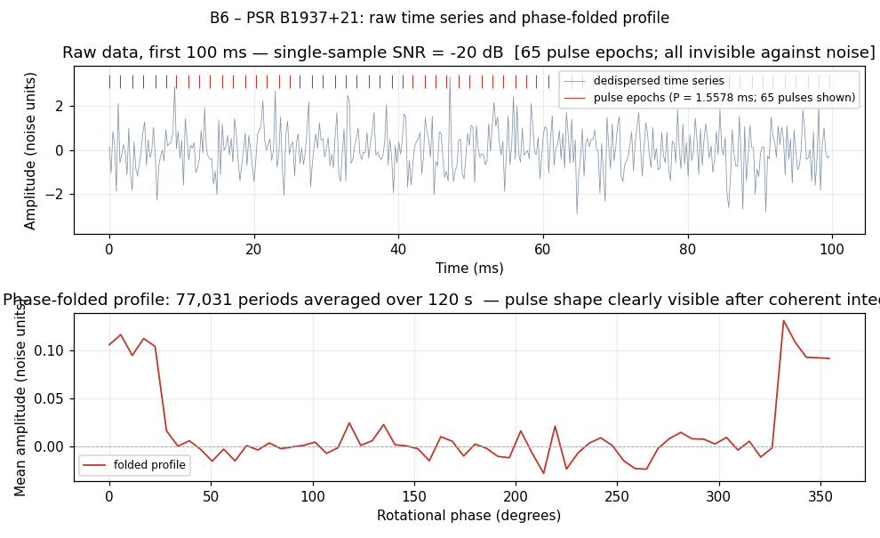
Top panel: first 100 ms of a simulated PSR B1937+21 dedispersed
time series (sample rate FS = 4,096 Hz). Signal amplitude = 0.1 × noise
sigma; single-sample power SNR = −20 dB. The sixty-four pulse epochs in
this window (red tick marks) are completely invisible against the noise
floor. Bottom panel: the same 120-second dataset phase-folded into 64
phase bins, averaged over 77,031 rotation periods. The pulse profile is
clearly visible after coherent integration — the same data, reorganised
by the algorithm.
The noise is the starting condition. What changes it is patience,
applied mathematically.
The resource: time, spent
patiently
The Fourier transform detects periodicity by an act of structured
addition. For each candidate frequency f, it asks: if I assume the
signal repeats at f, and I add together all the samples from periods
where the signal would be at its peak, do they reinforce or cancel? For
a purely random noise sample at frequency f, the answer is cancel — the
noise has no preferred phase, so positive and negative contributions
balance. For a signal that genuinely repeats at f, the answer is
reinforce — every period contributes positively to the same frequency
bin.
The mathematics of this SNR accumulation has a clean form:
SNR_amplitude ∝ sqrt(T_obs)This is the √T law. Double the integration time;
gain 3 dB in amplitude SNR. Increase it by a factor of 100; gain 10 dB.
Every 10 dB of additional signal burial costs a factor of 100 in
integration time. The resource you spend is not hardware, not
transmission power, not a cleverer algorithm. It is time — time during
which the periodic signal accumulates coherently in the Fourier
transform’s bookkeeping while the noise spreads across thousands of
frequency bins, diluting itself.
The code that implements this:
N    = len(time_series)
spec = np.fft.rfft(time_series)        # DFT
freq = np.fft.rfftfreq(N, d=1.0 / FS) # frequency axis
mag  = np.abs(spec) / N               # normalised magnitude
These are the same three lines — literally the same numpy calls —
that appear in every preceding chapter of the engineering guide this
post draws from: the analysis of an RLC circuit oscillation, a vibrating
industrial shaft, a radar echo. The DFT does not know it is processing a
pulsar. It measures, without any concern for the physical origin of its
input, which sinusoidal components are present and at what amplitude.
What changes, the only thing that changes between analysing a lab
oscillation and analysing a dead star, is N: the number of samples. In
B1 (the RLC circuit), N was 5,000. Here, N is 491,520.
The sense of scale this
requires
We should stop here, because a number needs to be held for a
moment.
A companion post on this site —
concerning the spin dynamics of a spacecraft measured by a probe fifty
metres away — applied the same Fourier transform to a signal that
crossed the approximate length of a car park. This post applies it to a
signal that has been travelling for 11,750 years. The source emitting
that signal has a radius of ten kilometres and an equatorial surface
velocity of 14% of the speed of light.
The algorithm is identical.
np.fft.rfft is not metaphorically or approximately the
same algorithm at both scales. It is the same algorithm. The same
floating-point operations, in the same order, on a time series that
could have originated from a lab instrument or from a neutron star in
Vulpecula. The mathematical structure does not care about the physical
substrate.
This is the scale-spanning quality of the Fourier transform that the
zemla.org series has been building toward. The algorithm in the radar
chapter (B5) extracted a weather target from 0 dB above the noise floor
across 64 milliseconds. Here, the same algorithm extracts a target from
20 dB below the noise floor across 120 seconds. Nine orders of
magnitude difference in source brightness; six orders of magnitude
difference in observation time; identical mathematical form.
The capacity for surprise this ought to produce is not always
proportional to the numbers. But the numbers are exact.
What the spectrum shows
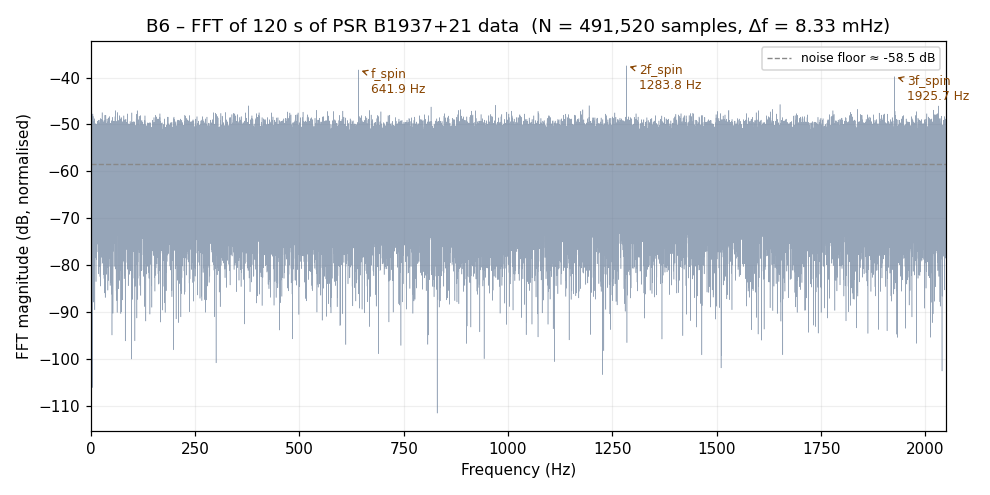
FFT magnitude of 120 seconds of simulated PSR B1937+21 data (N =
491,520 samples, Δf = 8.3 mHz). Three spikes are visible above the noise
floor: the spin fundamental at 641.9 Hz and harmonics at 1283.8 Hz and
1925.7 Hz. The fourth harmonic at 2567.6 Hz exceeds the Nyquist limit
(2048 Hz) and is absent. The narrow pulse width — each pulse is
approximately a single-sample spike — means the pulse train has
significant harmonic content, exactly as a square wave has odd
harmonics.
Running 120 seconds of observation through the Fourier transform
produces this picture. The frequency resolution is Δf = 1/T_obs = 1/120
= 8.3 mHz. The spike at 641.9 Hz is in bin k = 641.9 × 120 = 77,028. The
fractional frequency precision — from a single two-minute observation —
is Δf/f = 0.0083/641.9 ≈ 1.3 × 10⁻⁵.
The SNR growth follows the theoretical √T curve:
| Integration time | Samples (N) | SNR at f_spin |
|---|---|---|
| 1 s | 4,096 | 0 dB |
| 4 s | 16,384 | +6 dB |
| 16 s | 65,536 | +12 dB |
| 64 s | 262,144 | +18 dB |
| 120 s | 491,520 | +21 dB |

Top panel: FFT spectrum zoomed to the 580–720 Hz region after 120
s integration; the spike at 641.9 Hz is labelled with its peak SNR above
the noise floor. Bottom panel: measured SNR of the 641.9 Hz bin versus
integration time T (open circles, one simulation realisation), overlaid
on the theoretical √T curve (solid line). The dashed reference marks SNR
= 0 dB.
A signal that was −20 dB below the noise in any individual sample
becomes marginally detectable at T = 1 s and reaches a comfortable +21
dB margin at T = 120 s. A decade-long coherent timing campaign — the
kind the NANOGrav collaboration runs — narrows the frequency resolution
to Δf = 31.7 nHz, reaching sub-nanosecond timing residuals. This is how
~100-ns timing precision is achieved: the same three lines of code, run
on vastly more data, with careful correction for the pulsar’s spin-down,
its binary orbital motion, and the propagation delay through the
interstellar medium.
When the source
moves: the Hulse-Taylor binary
In 1974, Russell Hulse and Joseph Taylor, surveying pulsars with the
Arecibo telescope, discovered that the timing residuals of PSR B1913+16
— a pulsar spinning at 59.03 ms — contained a periodic modulation that
the best-fit spin-down model did not account for. The period of that
modulation was 7.75 hours (27,907 seconds). The pulsar was in a binary
orbit with a companion neutron star.
As PSR B1913+16 moves through its orbit, its distance from Earth
changes: closer during approach, farther during recession. Each arriving
pulse has therefore travelled a slightly different path length than the
preceding one, shifting the observed pulse arrival times earlier or
later by up to several light-seconds over one orbital period. The FFT of
the timing residuals — observed arrival times minus the best-fit
spin-down model — reveals a peak at the orbital frequency:
f_orbital = 1 / 27,907 s = 35.8 µHzThis is the Doppler measurement from the radar chapter, applied at a
timescale 10⁸ times longer. The DFT of pulsar timing residuals is
detecting a phase modulation at the orbital frequency in exactly the
same way the range-Doppler DFT in weather radar detects a phase
modulation at the Doppler frequency produced by a moving storm cell. The
mathematics is identical. The timescales are eight orders of magnitude
apart.
Hulse and Taylor received the Nobel Prize in Physics in 1993 for
characterising this orbit. The orbital period has been shrinking at
precisely the rate predicted by general relativity for a system losing
energy to gravitational radiation — the first indirect evidence that
gravitational waves exist, twenty-one years before LIGO detected them
directly.
A footnote: LIGO’s first gravitational-wave detection (GW150914,
September 2015) used a matched-filter pipeline — known template waveform
cross-correlated with the detector output in the frequency domain — that
is structurally the radar pipeline. The algorithm did not change between
detecting storm cells and detecting merging black holes.
Two telescopes, one
image: aperture synthesis
The range-Doppler map in radar was a two-dimensional DFT — range on
one axis, velocity on the other. Radio astronomy has its own
two-dimensional extension.
When two radio telescopes observe the same source simultaneously,
separated by a baseline of physical length b, the cross-correlation of
their recorded signals — called the visibility — is one sample
of the 2D Fourier transform of the sky’s brightness distribution. The
spatial frequency coordinates sampled are (u, v) = b/λ. As the Earth
rotates, the projected baseline traces an arc through the (u, v) plane.
A 27-antenna array like the Karl G. Jansky Very Large Array (named, in
1999, for the engineer who discovered the galaxy’s radio emission)
produces 351 distinct baselines simultaneously; after a full Earth
rotation it has sampled enough of the Fourier plane that an inverse 2D
FFT reconstructs a high-resolution image of the source.
This is aperture synthesis. The first event-horizon image of M87,
released in 2019 by the Event Horizon Telescope collaboration, was
reconstructed from visibility data recorded on eight radio telescopes
across four continents and Antarctica — an effective baseline equal to
the diameter of the Earth. The core mathematical operation was
np.fft.ifft2.
For the technically curious
The simulation that generated all three figures in this post runs in
under five seconds:
git clone https://github.com/lege-artis/fourier.git
cd fourier/examples/shad/b6-radioastronomy
pip install numpy matplotlib
python main.py
To observe the √T law directly: change T_OBS on line 32
of main.py from 120 to 60 and re-run. The spin-frequency
SNR drops by 3 dB. Change it to 240 and it rises by 3 dB. The √T
relationship is exact; the simulation makes it visible in real time.
Real pulsar data: the NANOGrav 15-year dataset — timing residuals for
68 millisecond pulsars — is publicly available (Agazie et al. 2023; data
at zenodo.org/records/8433091). The ATNF Pulsar Catalogue contains
parameters for all ~3,600 known pulsars at atnf.csiro.au/research/pulsar/psrcat.
The NANOGrav collaboration’s ongoing work to detect the stochastic
gravitational-wave background using pulsar timing arrays is at nanograv.org.
The broader engineering guide — from DFT foundations through
vibration diagnostics, radar, radioastronomy, and beyond-Fourier methods
— is at lege-artis/fourier.
What we heard, and what it
means
Let us try to say clearly what has happened here, because the
individual facts are familiar but their combination is, we think,
underappreciated.
We began with a signal. It originates 11,750 light-years from Earth,
from an object the size of a small mountain rotating 641.9 times per
second. When it arrives at a radio dish, its amplitude is one-tenth of
the background noise. In any one sample — any single measurement in the
time series — it is invisible. Not faint. Not marginal. Invisible. There
is no threshold of attention or instrument precision that isolates it
from the noise.
And then we wait. One hundred and twenty seconds. We accumulate
491,520 samples. We apply three lines of NumPy to the result. The
Fourier transform sorts the samples by frequency — asks, for each
possible frequency, how strongly is this frequency present? — and the
signal, which has been contributing the same phase to the same frequency
bin for 77,031 complete rotations, rises 21 dB above the noise floor.
The noise, which has been contributing incoherently to all frequency
bins, has averaged toward zero everywhere except where signals live.
This works because of a mathematical fact that has nothing to do with
astronomy: a signal that repeats at frequency f for T seconds
concentrates its energy into a frequency bin of width 1/T. The longer
the observation, the narrower the bin, the more the signal stands above
the noise distributed across all the other bins. The Fourier transform
implements this geometric fact. It does not know what a pulsar is. It
does not know what radio waves are. It measures periodicity, wherever
periodicity exists.
Three lines of numpy. Nine orders of magnitude in signal strength
from radar echo to pulsar, before integration. The algorithm did not
change.
There is a temptation, when confronted with this, to call it
beautiful and move on. What is remarkable is not just that mathematics
works at multiple scales. What is remarkable is the specific chain: a
tool devised to understand oscillating circuits, formalised to process
seismographic data from nuclear test monitoring, accelerated into the
fast Fourier transform by Cooley and Tukey in 1965, applied to radar
signal processing — this same tool, the same algorithm in the same
software library, now pulling a neutron star’s rotation from the
noise.
Karl Jansky was fixing a telephone problem. The people who used his
work to build Arecibo were not trying to detect gravitational waves. The
people who used the FFT for radar were not trying to image a black hole.
And yet: from Jansky’s rotating antenna to the Event Horizon Telescope’s
first M87 image is a chain of tools, each built for a different problem,
each reusable for problems its builders did not anticipate.
Mathematics, at its most generative, does not care what it is applied
to. That indifference is the whole point.
References
-
D. C. Backer, S. R. Kulkarni, C. Heiles, M. M. Davis, W. M. Goss,
“A millisecond pulsar,” Nature 300, 615–618 (1982). doi:
10.1038/300615a0. (Discovery of PSR B1937+21.) -
K. G. Jansky, “Electrical disturbances apparently of
extraterrestrial origin,” Proceedings of the Institute of Radio
Engineers 21, 1387–1398 (1933). -
R. N. Manchester, G. B. Hobbs, A. Teoh, M. Hobbs, “The Australia
Telescope National Facility Pulsar Catalogue,” Astronomical
Journal 129, 1993–2006 (2005). doi: 10.1086/428488. Available at
atnf.csiro.au/research/pulsar/psrcat. -
J. H. Taylor and J. M. Weisberg, “A new test of general
relativity — gravitational radiation and the binary pulsar PSR 1913+16,”
Astrophysical Journal 253, 908–920 (1982). doi: 10.1086/159690.
(Hulse-Taylor binary; first indirect gravitational-wave
evidence.) -
G. Agazie et al. (NANOGrav Collaboration), “The NANOGrav 15-year
data set: observations and timing of 68 millisecond pulsars,”
Astrophysical Journal Supplement 265, 49 (2023). doi:
10.3847/1538-4365/acdc91. Data at zenodo.org/records/8433091. -
D. R. Lorimer and M. Kramer, Handbook of Pulsar
Astronomy, Cambridge University Press,- ISBN 0-521-82823-6.
