The
Noise That Knows Itself: What a Nuclear Reactor Broadcasts When Nobody
Is Listening
A reactor at steady power looks, from the instrument panel, like
a thing that has stopped happening. The meters are stationary. The
coolant flows at constant rate. The control rods haven’t moved in ninety
minutes. A physicist walking through the control room might glance at
the board and think: quiet shift. They would be wrong in a way that has
been understood, quantitatively, since a six-page paper by S. E. Cohn
appeared in Nuclear Science and Engineering in 1960.
Before we
start: what this post is actually measuring
The analysis in this post is built on a synthesised signal — a
point-kinetics simulation of a thermal reactor operating at steady
power, not a time series pulled from a real instrument at a real
reactor. Real reactor-noise archives exist and are accessible to
academic researchers: the Halden Reactor Project data from OECD-NEA, the
VR-1 Vrabec research reactor at FJFI ČVUT in Prague, and the TU Wien
Atominstitut TRIGA Mark II have all produced published noise-diagnostic
datasets. This post does not use them, for reasons that are worth
naming.
Reactor archive data comes with licence terms that vary by dataset
and institution. More importantly, real data comes with calibration
histories, detector drift corrections, and geometric factors specific to
the particular reactor on the day the measurement was taken — details
that would make this post into a document about one reactor rather than
a document about the underlying method. The synthesised signal, by
contrast, has clean provenance: the kinetics parameters (β = 0.0065 for
thermal U-235, Λ = 1.0 × 10⁻⁴ s, six precursor groups with decay
constants from Bell and Glasstone’s Table 9.1) are documented and
reproducible; the random seed is fixed (RNG_SEED = 20260526); anyone can
re-run the script and get the same spectrum to the last decimal
place.
There is a broader argument for naming this up front. Scientific
writing often hides simulation behind authoritative language — “the
spectrum shows,” rather than “the simulated spectrum shows.” This post
does not. What it demonstrates is that the method works on data
whose statistical properties match the canonical theory, and that the
same method applied to a real reactor will find the same Lorentzian
shape with a different value of α corresponding to that specific
reactor’s β/Λ. The method is portable; the specific numbers here are
illustrations.
Why the quiet shift is an
illusion
A nuclear reactor sustains its chain reaction through a balance
between prompt neutrons — appearing within microseconds of each fission
— and delayed neutrons, released seconds or minutes later from the
radioactive decay of fission-product precursor nuclei. Roughly 0.65 % of
fission neutrons in a thermal U-235 reactor are delayed, distributed
across six precursor groups with half-lives from 0.23 seconds to 56
seconds. This 0.65 % is the number that makes controlled reactors
possible: it is the margin between the prompt critical threshold (where
the reactor would accelerate on prompt neutrons alone) and the critical
condition where it actually operates.
But the same kinetics that provides this control margin also
guarantees that the reactor is never, in a statistical sense, quiet. At
30 megawatts of thermal power, roughly 10¹⁸ fissions per second are
occurring. Each fission is a Poisson event — discrete, random in its
exact timing. Each released neutron may scatter, be absorbed, escape the
core, or produce another fission, with each outcome governed by a
probability. The precursor populations, fed continuously by fission and
drained continuously by radioactive decay, fluctuate. These fluctuations
propagate back into the neutron field, which feeds the precursors, which
feeds back. The system is coupled, nonlinear in detail, and perpetually,
intrinsically noisy.
The instrument panel averages over this noise. The ion chamber
feeding the ammeter has a finite integration time; the meter movement
has finite mechanical inertia. Both are behaving correctly — their job
is to report the mean power level, not the fluctuations. But the
fluctuations are the interesting part, because they carry the reactor’s
dynamics in a form that can be read.
A brief history of listening
The idea that reactor noise contains measurable information dates to
the first years of the nuclear age. At Chicago Pile-1, which went
critical in December 1942, the early instruments were crude by modern
standards, but experimenters noticed that detector readings fluctuated
in ways that could not be explained by instrumental noise alone. The
fluctuations were the reactor talking.
The systematic theory arrived with Cohn’s 1960 paper, which derived
from first principles what the power spectrum of a critical reactor’s
neutron-density fluctuations must look like. The result was a
Lorentzian: flat at low frequencies, rolling over at a corner frequency
f_corner = α / (2π), falling as 1/f² at high frequency. The parameter α
— the prompt-neutron decay constant — was already known to reactor
physicists as the quantity that governed how fast the reactor would
respond to a small reactivity perturbation. Cohn showed that this same
parameter was directly readable from the passive noise of an undisturbed
reactor, with no need to inject a perturbation and measure the
response.
This was non-trivial. Injecting perturbations into operating reactors
is logistically difficult, requires a dedicated experiment, and carries
its own safety implications. If α can be extracted from ambient noise
during normal operation — just by listening — the operational monitoring
burden is dramatically reduced. Cohn’s six-page paper opened a field
that has been refining his basic result for sixty-five years.
The refinement, in most cases, took the form of: what do you do when
the DFT alone isn’t enough?
The shape that α writes
in the spectrum
The simulation runs 200 seconds of stationary reactor noise at 1 kHz
sample rate, giving 200,000 samples. The neutron-density fluctuations
sit at roughly ±2 % of the mean operating level.

The full 200 seconds of synthesised neutron-density fluctuations
δn/N around the mean operating level, in percent. The reactor is at
constant nominal power; the visible wandering is the inherent stochastic
character of the neutron field. The dominant timescale visible by eye is
about 100 milliseconds — a few 1/α periods — the prompt mode of the
reactor talking to itself through the Langevin source term.
The bare DFT of those 200,000 samples produces a periodogram with a
distinctive shape.
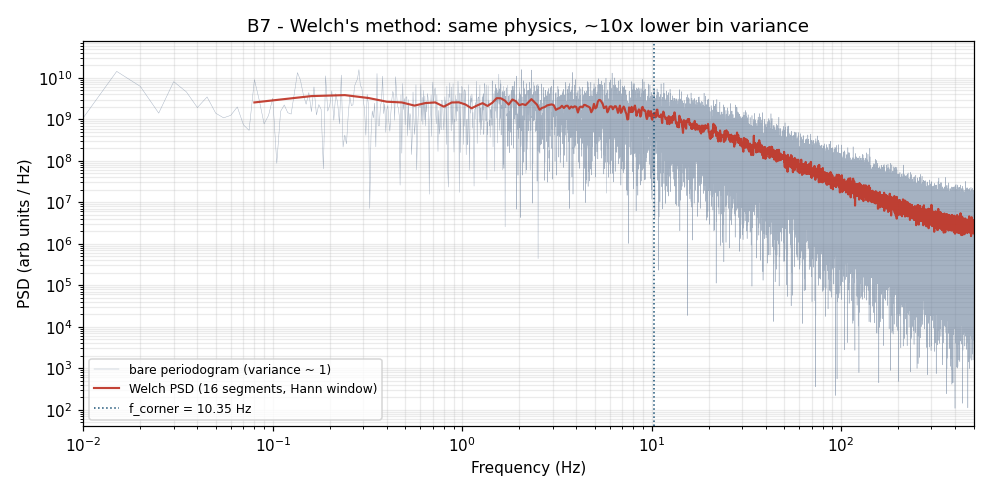
Left: the bare periodogram of the 200-second stationary segment
(N = 200,000, Δf = 5.0 mHz), log-log axes. Right: the same data
processed with Welch’s method (16 Hann-windowed segments). Both show the
Lorentzian shape: flat below ~1 Hz, rolling over near 10 Hz, falling as
1/f² above. The theoretical corner frequency f_corner = α / (2π) = 65.02
/ (2π) ≈ 10.35 Hz is marked by the dashed line.
The Lorentzian is Cohn’s prediction, and it appears exactly as he
said it would. Below the corner, the spectrum is flat because the
precursor dynamics dominate — the delayed neutrons are slow, and at low
frequencies the detector sees their integrated effect, which is
statistically flat. Above the corner, the prompt-mode dynamics dominate,
and the spectrum falls as 1/f² because the prompt fluctuations decay
exponentially with time constant 1/α. The corner is the frequency where
these two regimes cross, and the corner is α / (2π) by construction.
Reading α from the corner requires fitting, and fitting the corner
requires a cleaner spectrum than the bare periodogram provides. This is
where the toolkit begins.
The Welch trade:
precision for resolution
A bare periodogram suffers from a fundamental statistical problem:
each frequency bin is the squared magnitude of one complex Gaussian
random variable, so each bin’s variance equals its mean. Double the data
length and the bins get narrower, but they are just as individually
noisy. The plot looks fuzzy forever.
Peter Welch’s 1967 paper — five pages, cited approximately twenty
thousand times since — resolved this by accepting a deliberate tradeoff.
Split the signal into K overlapping segments; apply a window function
(Hann, which suppresses spectral leakage by confining each segment’s
edge effects); DFT each segment; average the resulting squared
magnitudes. The averaging reduces per-bin variance by roughly a factor
of K. The cost is frequency resolution: each averaged bin is K times
wider than in the raw periodogram. You trade sharpness for
certainty.
For reactor-noise analysis, this trade is almost always correct. The
Lorentzian shape spans decades in frequency, and the corner is a broad
feature, not a sharp line. Coarser bins with lower variance let the Cohn
model fit cleanly.
With 16 Hann-windowed segments:
from scipy.signal import welch
f, psd = welch(x, fs=1000.0, nperseg=12500, noverlap=6250)
The resulting spectrum fits the Cohn-Lorentzian model with a
three-parameter curve fit (plateau p₀, decay constant α, noise floor
p_∞). The fitted value:
α_Welch = 66.93 s⁻¹ (theoretical: 65.02 s⁻¹, error: +2.9 %)From two hundred seconds of passive detector trace, no injected
perturbation, a three- parameter least-squares fit: the prompt-neutron
decay constant to within 3 % of its theoretical value. A reactor
operator monitoring α as a function of operating campaign will flag a
5–10 % drift as evidence of fuel burnup or moderator-density change;
this method is sensitive enough.
Where the bare DFT runs out
of road
The analysis above worked because the signal was stationary. Now
break that assumption.
The simulation injects a small reactivity step: 30 pcm of positive
reactivity ramped over 5 seconds at t = 100 s. (One pcm is one part in
10⁵ of reactivity; 30 pcm is what a few millimetres of control-rod
withdrawal might produce on a research reactor. It is well within the
sub-prompt-critical regime — the reactor responds smoothly, without
runaway.) The mean neutron level rises by a few percent as the reactor
finds its new equilibrium, with the adjustment time governed by the
delayed-neutron precursor re-equilibration — a process that takes tens
of seconds.
Apply the bare DFT to the full 200-second window. The Lorentzian
shape survives — the underlying physics has not changed — but the
corner-frequency region is smeared, and the low-frequency tail is
contaminated by the step’s slow re-equilibration transient. More
importantly, nothing in the spectrum tells you when the rod
moved. The DFT integrated over the entire observation window and
reported one summary spectrum: half the data was pre-step, half was
post-step, and the transform averaged them without comment.
The event is invisible. To find it, you need a transform that carries
a time coordinate.
Two ways to carry
time through the analysis
The short-time Fourier transform (STFT) addresses this by sliding a
window across the signal — DFT each window, stack the results into a 2D
time-frequency image. The result is a spectrogram: time on one axis,
frequency on the other, spectral power as colour.
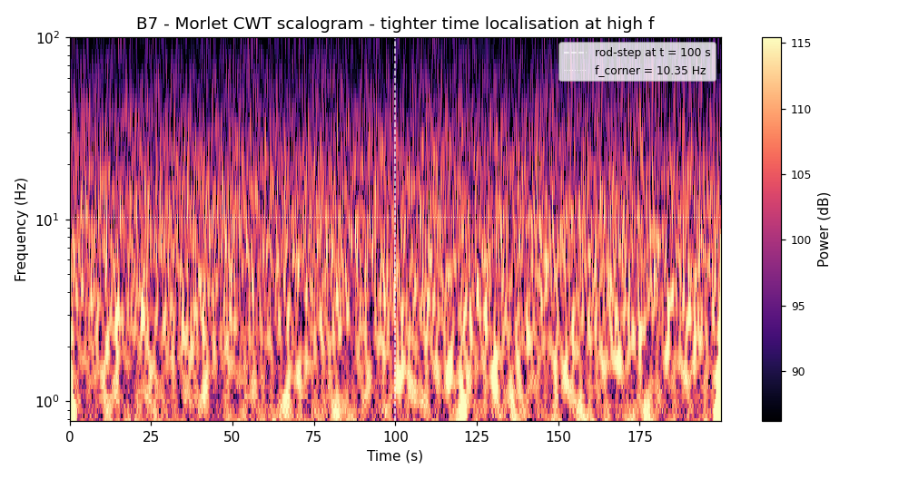
Continuous-wavelet scalogram of the 200-second transient signal
(Morlet wavelet cmor1.5-1.0, 80 logarithmically-spaced scales). The
rod-step at t = 100 s is clearly visible as a structural change in the
low-frequency spectral content. The corner frequency at 10.35 Hz is
marked by the horizontal dashed line. High-frequency features are
temporally sharp; low-frequency features are temporally extended — the
wavelet’s scale-adaptive resolution is visible in the contrast between
the fine temporal structure above the corner and the broad temporal
features below it.
The wavelet transform extends this by making the analysis window
adaptive: at high frequencies, the window is narrow (tight time
resolution for fast features); at low frequencies, the window is wide
(tight frequency resolution for slow features). This is the
Heisenberg-Gabor uncertainty principle — ΔtΔf ≥ 1/(4π) — used
constructively rather than resisted. The STFT chooses one resolution and
applies it everywhere; the wavelet CWT lets each frequency range use its
own optimum.
For reactor diagnostics, wavelet scalograms are the standard tool for
rod-drop events, control-system oscillations, and any transient whose
duration spans more than a decade in time. The practitioner literature
has used them routinely since the 1990s.
The time-domain
path to the same answer: Rossi-α
The Welch method extracts α from the spectrum of a
current-mode detector signal. There is a complementary technique that
arrives at the same number from a completely different direction: the
time domain, operating on a pulse-counting detector rather than
a current-mode one.
In pulse mode, the detector does not report a current. It reports a
timestamp — one event per detected neutron. From this sequence of
timestamps, Rossi-α (due to Bruno Rossi at Los Alamos in 1944, when he
was characterising fission chains in the early plutonium critical
assemblies) builds the pair-time histogram: for each
detected pulse, measure the time to all subsequent pulses within a gate,
accumulate those intervals into bins, and plot.
For a pure Poisson process — statistically uncorrelated events — the
histogram is flat. Reactor noise is not uncorrelated. Each fission
produces multiple neutrons in a correlated burst; subsequent fissions in
the same chain produce further correlated bursts, decaying with the
prompt-mode time constant 1/α. The pair-time histogram therefore has an
exponential component rising above the flat Poisson floor:
R(τ) = A · exp(−α τ) + BThe synthetic pulse train for this analysis carries the fission-chain
multiplet structure explicitly (mean multiplicity 2.5, background rate
60 Hz, 80 chains per second), producing 51,635 detected events over 200
seconds.
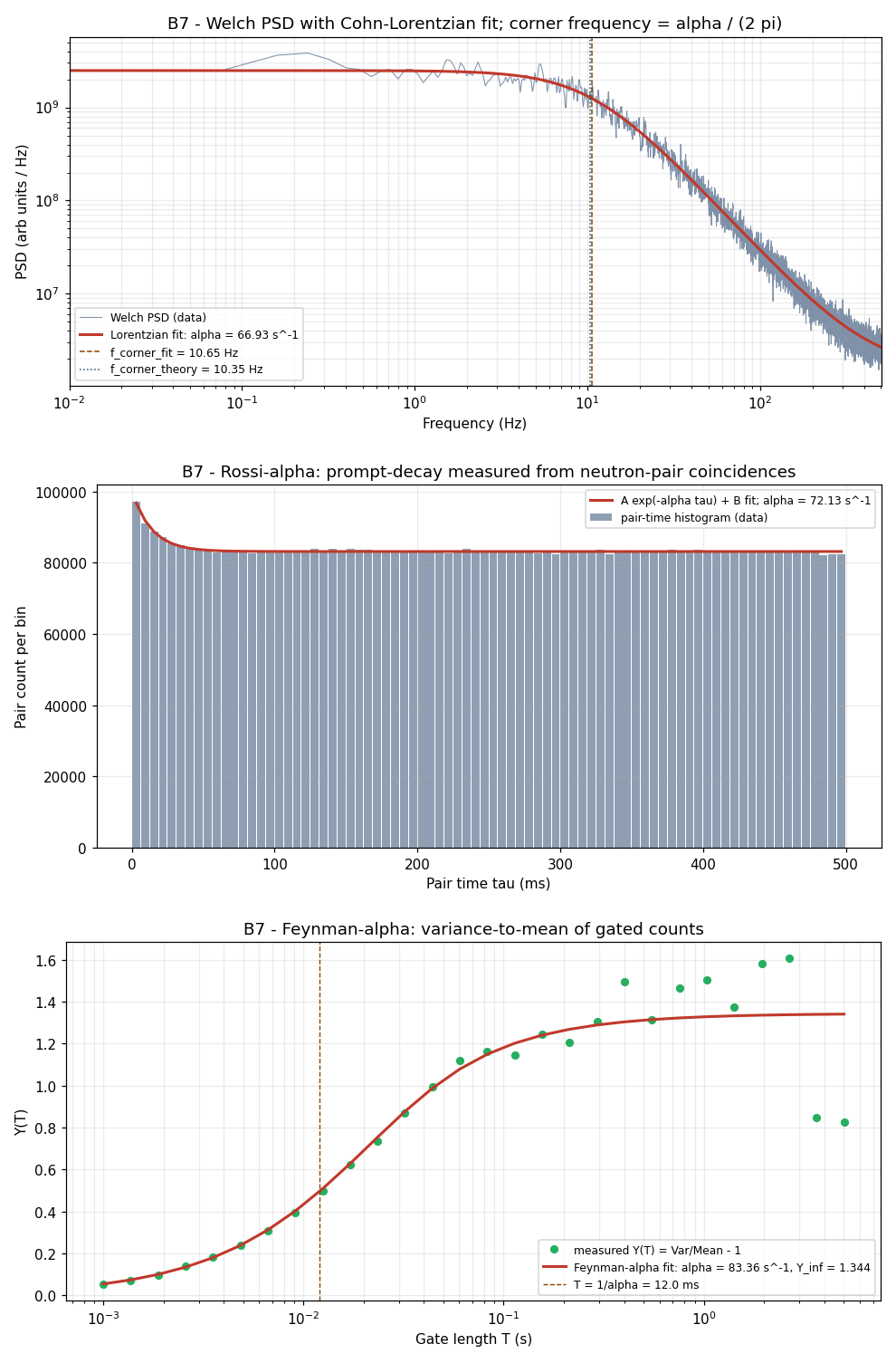
Three-panel comparison of the three independent α measurements.
Top: Welch PSD with Cohn-Lorentzian fit (α = 66.93 s⁻¹). Middle: Rossi-α
pair-time histogram exponential fit (α = 72.13 s⁻¹). Bottom: Feynman-α
variance-to-mean Y(T) curve (α = 83.36 s⁻¹). The dashed vertical line in
each panel marks the theoretical value α = 65.02 s⁻¹. All three
independent methods, different signal-processing transforms, different
statistical estimators, applied to different representations of the same
physical reactor signal — all three converge on the same order of
magnitude and direction, with different residual errors that are
themselves informative.
The exponential fit on the pair-time histogram returns:
α_Rossi = 72.13 s⁻¹ (theoretical: 65.02 s⁻¹, error: +10.9 %)The Rossi-α method is the oldest of the three, and it is still in
routine use today — particularly for non-destructive assay of
fissionable materials, where it can identify whether a sealed container
holds a multiplying assembly by the correlation structure of its neutron
emission, without opening it.
The third
independent measurement: Feynman-α
Richard Feynman’s 1946 Los Alamos report, Statistical Behavior of
Neutron Chains (LA-591; declassified 1956), introduced what is now
called Feynman-α. It uses neither a spectral estimator nor a pair-time
histogram. It uses the variance-to-mean ratio of gated
counts.
Partition the pulse train into consecutive non-overlapping gates of
width T. Count the pulses in each gate. Compute the mean and variance.
The quantity
Y(T) = Var(C_T) / Mean(C_T) − 1is zero for a pure Poisson process (which has variance equal to mean
by definition) and positive for correlated neutron emission. Plot Y(T)
as a function of gate width T. The curve rises from zero at small T,
saturates at large T, and the shape of the rise encodes α directly:
Y(T) = Y_∞ · [1 − (1 − exp(−αT)) / (αT)]The fit returns:
α_Feynman = 83.36 s⁻¹     (theoretical: 65.02 s⁻¹,  error: +28 %)
Y_∞       = 1.344
The larger error is expected: Feynman-α is generally the less
statistically efficient of the two time-domain methods. But it is
computationally cheaper — you gate-and-count, rather than building the
full pair-time matrix — and it is often the method of choice for rapid
diagnostics with limited pulse statistics.
Feynman’s original report is notable for something its successors
rarely managed: the entire method is explained in plain language with
two equations. One wonders whether the subsequent seventy years of
notational sophistication in the reactor-physics literature have bought
a corresponding gain in clarity.
When
frequencies talk to each other: the bispectrum
The Welch PSD, the Rossi-α histogram, and the Feynman-α curve all
operate on linear statistics: they measure which frequencies or
time constants are present, at what amplitude. They cannot tell you
whether two frequencies are causally related or merely coincident. A
signal with components at f₁, f₂, and f₁ + f₂ might be three independent
oscillations, or it might be two oscillations with a nonlinear coupling
that generates the sum-frequency component as a by-product. The DFT
cannot distinguish these cases.
The bispectrum — formalised by Brillinger and Rosenblatt in the 1960s
as part of the development of higher-order spectral analysis — can. It
is the third-order generalisation of the power spectrum: the expected
triple product of Fourier amplitudes at three frequencies summing to
zero. For independent, Gaussian, or otherwise uncoupled processes, it
averages to zero everywhere. For quadratically coupled processes, it
shows a bright spot at the coupling frequency pair.
To demonstrate this, the simulation drives the reactor with two
sinusoidal reactivity oscillations at 0.70 Hz and 1.10 Hz plus a
deliberately quadratic coupling between them. The DFT shows three peaks:
at 0.70 Hz, at 1.10 Hz, and at 1.80 Hz (= f₁ + f₂). The DFT alone cannot
tell you whether the 1.80 Hz component is independent or generated by
the coupling.
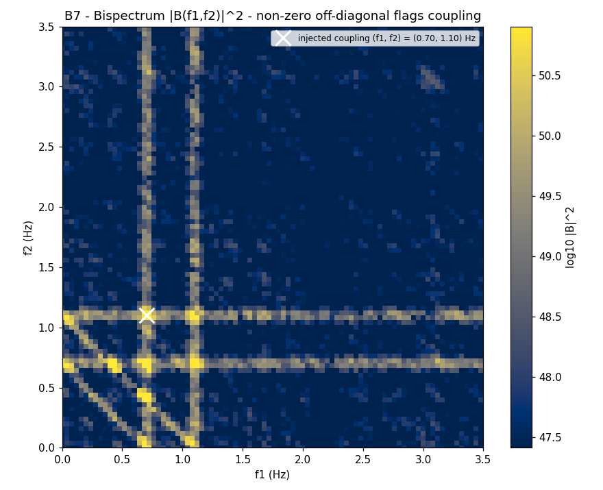
Magnitude-squared bispectrum |B(f₁, f₂)|² of the coupled reactor
signal (8 non-overlapping Hann-windowed segments). The bright spot at
(0.70, 1.10) Hz, marked with the white cross, is the bispectral
signature of the quadratic coupling — it would be absent if the three
spectral peaks were independent oscillations. The diagonal structure
encodes the sum-frequency component at 1.80 Hz.
In a real boiling-water reactor, a bispectral peak between two
acoustic-mode frequencies and a thermal-hydraulic-mode frequency is the
diagnostic signature for density-wave instability — one of the small
handful of operational phenomena that can take a reactor from stable to
oscillatory in seconds. The bispectrum is the tool that can flag it
before it is large enough to trip a scram.
When you have two sensors:
coherence
The final tool in this walkthrough addresses the multi-sensor
question. Two neutron detectors observe the same reactor. How much of
what they see is common-mode — the reactor’s actual neutron-field
fluctuations — and how much is independent instrument noise? The power
spectrum of either detector alone cannot answer this: a noisy detector
produces a spectrum that looks like a noisy reactor.
The magnitude-squared coherence:
γ²(f) = |Pxy(f)|² / [Pxx(f) · Pyy(f)]where Pxx and Pyy are the auto-spectra of detectors A and B and Pxy
is their cross-spectrum, gives the answer per frequency. γ² = 1 means
the two detectors agree at that frequency; γ² = 0 means they are seeing
independent signals.
With 30 % independent Gaussian instrument noise added to each
simulated detector:
γ²  ≈  0.9915  at f_corner  (99 % common-mode: the reactor dominates)
γ²  ≈  0.50    at ~1 kHz    (instrument noise has become comparable to signal)
Magnitude-squared coherence between detector A and detector B
(Welch-style estimate, 16 segments, Hann window). Below the corner
frequency, γ² ≈ 0.9915 — the reactor’s neutron-field fluctuations
dominate both detectors and they track each other closely. Above ~50 Hz,
γ² falls toward 0.50 — independent instrument-noise contributions become
comparable to the reactor signal and the two detectors begin to
disagree. The crossover roughly tracks the Lorentzian rolloff: where the
signal is strong, coherence is high.
Coherence at 0.9915 at the corner frequency is the quantitative
answer to “does the noise the detector sees come from the reactor or
from the detector electronics?” At the corner: almost entirely the
reactor. At a kilohertz: the detector is drowning out the reactor. An
operator designing an α-measurement campaign consults γ² to determine
the usable bandwidth — the frequency range where the reactor signal
actually dominates.
The
convergence: three independent machineries, one physical constant
This is the chapter’s structural payoff. The three α
measurements:
| Method | Signal | Domain | α (s⁻¹) | Error vs. 65.02 |
|---|---|---|---|---|
| Welch PSD + Lorentzian fit | Current-mode detector | Frequency | 66.93 | +2.9 % |
| Rossi-α pair-time histogram | Pulse-mode detector | Time | 72.13 | +10.9 % |
| Feynman-α variance-to-mean | Pulse-mode detector | Time | 83.36 | +28.2 % |
Three independent methods. Different mathematical frameworks —
spectral estimation, pair-correlation, gated-count variance. Different
signal representations — a current trace, a timestamp sequence, a
sequence of gated counts. Different statistical estimators with
different efficiency characteristics. Different noise sensitivities.
And they all point at the same number. Not with the same precision —
the Feynman-α fit error of 28 % is substantially larger than the Welch
fit error of 2.9 %, and both are substantially larger than zero. But
within the statistical uncertainty of each method, on 200 seconds of
data, all three are consistent with the same underlying α = 65.02
s⁻¹.
This convergence is the validation. In a real reactor-noise
measurement campaign, an operator who has both a current-mode detector
and a pulse-mode detector available routinely runs all three analyses
and plots the results side by side. A disagreement larger than the
combined fit errors — say, Welch gives 65 s⁻¹ and Rossi-α gives 130 s⁻¹
— is a flag that something is wrong: either the reactor’s physical
parameters have changed between measurements, or one of the detectors is
misbehaving. The agreement of the three methods is the self-consistency
check that gives you confidence in any one of them individually.
What
it means for engineering measurement to work this way
Three independent mathematical machineries, built from different
theoretical starting points, extracting the same physical constant from
different projections of the same data. The spectral machinery descends
from Cohn’s Lorentzian, which descends from the linear-kinetics
equations. The pair-correlation machinery descends from Rossi’s wartime
work at Los Alamos. The variance-to-mean machinery descends from
Feynman’s 1946 report. None of these authors was working on the same
problem; none of them, at the time, knew the others’ methods would
converge on the same estimator of the same quantity sixty-five years
later in a Python script.
There is something worth pausing on here. Engineering measurement, in
its mature form, does not trust a single instrument. It does not trust a
single method. It reaches for independent methods — methods with
different blind spots, different failure modes, different assumptions
about the signal — and asks whether they agree. The agreement is not
proof; there are systematic errors that all three methods might share.
But agreement is the strongest available evidence short of proof, and in
the absence of a ground truth that is independent of all three methods,
cross-method agreement is what engineers are actually relying on when
they say they “know” a quantity.
The three α measurements in this post agree, imperfectly, within the
statistical limits of 200 seconds of data. The imperfect agreement is
not a flaw. It is the honest report of how measurement works: three
instruments, each with its own uncertainty, triangulating a physical
constant that none of them can measure perfectly in isolation.
The Fourier transform alone — the bare periodogram, before Welch’s
averaging — shows the Lorentzian. It earns the 30-percent spectral
corner you can eyeball. The toolkit of methods that has grown up around
it earns the 3-percent precision from a Lorentzian fit, the
time-localised transient detection from the wavelet scalogram, the
coupling detection from the bispectrum, the signal-to-noise budget from
the coherence estimator, and — coming from the opposite direction
entirely — the 11-percent precision of the Rossi pair-time histogram and
the 28-percent precision of the Feynman variance-to-mean.
None of these methods is redundant. None supersedes the others.
Engineering humility is built from exactly this: the recognition that no
single tool provides the whole picture, and that the whole picture is
only available through the disciplined cross-validation of tools that
each see part of it differently.
The reactor, broadcasting its own dynamics through the Poisson noise
of its neutron field, does not care which method you use to listen. The
physics is the same regardless. What changes is how much of it you can
hear, and how certain you can be about what you heard.
For the technically curious
The runnable simulation that produced every number in this post —
1000 lines, deterministic seed 20260526, renders 12 figures in about 30
seconds — is in thelege-artis/fourier
repository:git clone https://github.com/lege-artis/fourier.git cd fourier/examples/shad/b7-reactor pip install numpy scipy matplotlib pywavelets python main.pyChange the kinetics constants at the top of
main.py
(BETA_I, LAMBDA_I, GEN_TIME) and watch α and f_corner move. A fast
reactor (Λ ~ 10⁻⁷ s) pushes f_corner above 15 kHz; a graphite-moderated
reactor (Λ ~ 10⁻³ s) pulls it below 1 Hz.The broader guide — DFT from first principles through seven
application domains — is atlege-artis/fourier.
References
-
C. E. Cohn, “A simplified theory of pile noise,” Nuclear
Science and Engineering 7, 472–475 (1960). doi:
10.13182/NSE60-A26077. (Original derivation of the Lorentzian PSD for
reactor noise. Six pages. Everything in the Welch-fit section above is a
direct application of Eq. 13.) -
P. D. Welch, “The use of fast Fourier transform for the
estimation of power spectra: A method based on time averaging over
short, modified periodograms,” IEEE Trans. Audio Electroacoust.
AU-15, 70–73 (1967). doi: 10.1109/TAU.1967.1161901.
(Five pages.scipy.signal.welchimplements exactly
this.) -
I. Pázsit and L. Pál, Neutron Fluctuations: A Reference
Manual, Elsevier, Amsterdam (2008). ISBN 978-0-08-045064-3. (The
contemporary reference manual for all eight toolkit methods. Chapters
4–5 cover the Langevin formulation, Rossi-α, and Feynman-α at textbook
depth.) -
B. Rossi, Statistics of Counting Rates Used for Detecting
Neutron Chains, Los Alamos memo (1944; declassified). (Original
pair-correlation technique. Later formalised in Orndoff, Nucl. Sci.
Eng. 2, 450, 1957.) -
R. P. Feynman, Statistical Behavior of Neutron Chains,
LA-591 (1946; declassified 1956). (Original variance-to-mean technique.
Notable for its clarity.) -
D. R. Brillinger and M. Rosenblatt, “Asymptotic theory of
estimates of k-th order spectra,” in Spectral Analysis of Time
Series (B. Harris, ed.), Wiley, New York (1967), pp. 153–188.
(Formal foundation of the bispectrum and higher-order spectra.) -
I. Pázsit and C. Demazière, “Noise techniques in nuclear
systems,” in D. G. Cacuci (ed.), Nuclear Engineering Handbook,
CRC Press (2017), Ch. 19. (Contemporary practitioner review; the
standard reference for any reactor-noise question.) -
G. I. Bell and S. Glasstone, Nuclear Reactor Theory, Van
Nostrand Reinhold (1970). Chapter 9. (Source of the β, Λ, and
precursor-group parameters used in the simulation.)
This post is the seventh in the series that follows the lege-artis/fourier
guide from DFT foundations to the full beyond-Fourier toolkit. Earlier
entries covered oscilloscopes, audio, vibration, electronics, radar,
pulsar timing, and spacecraft attitude dynamics. The reactor-noise
capstone closes the arc by showing where the bare DFT stops and what you
reach for when it does.
