At 09:50:45 UTC on 14 September 2015, gravitational-wave astronomy was born. The LIGO gravitational-wave detectors recorded a signal (the European Virgo was not yet in full operation, and the LIGO detectors themselves, freshly upgraded, were only at the end of their test run — but that is another story) that the official catalogue of gravitational-wave events now lists as the first: GW150914. Its source was the final phase of the merger of two black holes with masses of the order of several tens of Suns. That in itself was something of a surprise. It was the first direct detection of gravitational waves. The data from both detectors are public — anyone can download them from the Gravitational Wave Open Science Center and try to find the signal themselves.
We did. The first attempt failed. The second worked. This text is about what happened in between — because that is where you see how much of detection is Fourier analysis, and how many mistakes you can make without touching the physics.
What the detector measures
A LIGO detector is a Michelson interferometer with four-kilometre arms. A gravitational wave stretches one arm very slightly and shortens the other; the result is one time series per detector, the strain h(t) — the relative change in arm length. For GW150914 it peaked around 10⁻²¹: a four-kilometre arm changed by the order of a thousandth of a proton’s diameter.
Across the whole band where the signal lives, the detector noise is comparable or larger. Around 100 Hz its density is about 10⁻²³ per root hertz; below 30 Hz it rises steeply (seismic), above a few hundred hertz it rises again (quantum noise of the light). On top of that, narrow spectral lines: 60 Hz mains and harmonics, violin modes of the mirror suspensions near 500 Hz, calibration lines. The signal sits below the noise — in the raw data you cannot see it.
First attempt: why nothing came out
We took a 32-second file around the event, did a single Fourier transform, divided it by a noise estimate from the same 32 seconds, and looked for a rising tone in a time-frequency map. The loudest spot was at 32–40 Hz, away from the merger time, with no „chirp“.
The fault was not in the data but in the method: a noise spectrum estimated from one transform has enormous variance (each frequency is estimated from two numbers), and 32 seconds is not enough for a decent estimate. The guide that the LIGO and Virgo collaborations published alongside the open data devotes a large share of its exposition to exactly this — estimating the noise.
What the collaboration does — and what we did the second time
The procedure the collaboration describes for displaying the signal has four steps:
- Noise spectrum as a median. From 1024 seconds of data around the event, spectra are computed in four-second windows shifted by two seconds (Welch’s method), and the median is taken, not the mean. The median does not let a single loud disturbance — or the signal itself — distort the spectrum.
- Window. The data are multiplied by a Tukey window before transforming. Without a window, the huge low-frequency noise „leaks“ into the whole spectrum.
- Whitening. The data spectrum is divided by the square root of the noise spectrum. This flattens the noise — every frequency gets equal weight, and a weak signal in a quiet band stops disappearing under loud noise elsewhere.
- Band-pass 35–350 Hz — for display only. The search itself does not use it.
We did this with the 4096-second files from both detectors. Result:
| what we measured | our result | published value |
|---|---|---|
| noise at 100 Hz | 9.2 × 10⁻²⁴ (H1), 9.9 × 10⁻²⁴ (L1) /√Hz | ≈ 10⁻²³ /√Hz |
| data quality around the event | all quality flags set in both detectors | same |
| whitened noise away from the event | standard deviation 1.005 and 1.008, excess kurtosis +0.05 and +0.04 | Gaussian: 1 and 0 |
| time lag between detectors | Livingston leads Hanford by 7.3 ms, signal sign inverted | 6.9 (+0.5/−0.4) ms, inverted sign |
| time of peak | 0.02 s after the catalogue time | merger ≈ 0.02 s after the catalogue time |
| frequency in the last 0.1 s (Hanford) | 39 → 52 → 84 → 175 Hz | rise from ~35 to ~250 Hz |
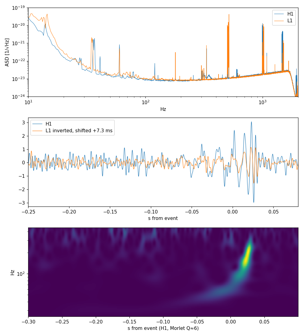
The 7.3 ms lag lies within the published interval. The inverted sign reflects the relative orientation of the two detectors‘ arms. And the bottom panel shows why the signal is called a chirp: in less than a tenth of a second the frequency sweeps from tens to hundreds of hertz as the black holes make their last orbits and merge.
Two errors in our own tools
We did not get there directly. Along the way we twice measured something that was not true — and both errors were in our checks, not in the data.
- The Gaussianity test at first reported massive failure. But it compared noise at a finer frequency resolution with a noise spectrum estimated at a coarser one. Where there is a narrow spectral line, the two resolutions do not match — and the test was measuring its own mismatch. At the same resolution as the noise spectrum, the noise comes out almost exactly Gaussian.
- Frequency tracking at first gave nonsense, because the time-frequency map had a resolution of 16 Hz — far too coarse for a signal that crosses hundreds of hertz in a tenth of a second. A wavelet transform with constant bandwidth-to-frequency ratio fixed it.
A third, similar experience — a check run on one segment of data instead of the whole file — is described separately on mim2000.cz.
Where Fourier sits in this
Not as one tool among many, but as the axis. Every step the collaboration takes, from whitening through search to parameter estimation, rests on one object: an inner product of signals in which each frequency is weighted by the inverse of the noise spectrum. It is simple only in the frequency domain, because stationary Gaussian noise has mutually independent Fourier coefficients. Window, median, whitening — all of it is care to make that condition hold well enough on real data.
What do we take from this in practice? Three conclusions, each modest and well supported.
- Public data suffice to reproduce the picture of the signal — even without specialised software. We needed numpy, scipy and h5py, 4096 seconds of data and the procedure the collaboration itself published. We did not thereby verify the detection (that requires a template filter and a background estimate); we reproduced its picture and four measurable properties.
- Estimating the noise is half of detection. The difference between „nothing“ and „a clear chirp“ was not in the signal but in how much data we used and how robustly we estimated the noise.
- A check has to be able to fail for the right reason. Both of our faulty checks would, without a second look, have passed for properties of the data. A check should first be tried on a case where the answer is known.
What next
The next step is the matched filter: correlate the data with the theoretical waveform from general relativity and measure the signal-to-noise ratio — the published value is about 24 for both detectors combined. There will be two templates, the official one and our simplified one, and both will first go through test cases where the answer is known from theory. Only then will they go to the data.
References
- Abbott, B. P. et al. (LIGO Scientific Collaboration and Virgo Collaboration) (2016). Observation of gravitational waves from a binary black hole merger. Physical Review Letters, 116, 061102. https://doi.org/10.1103/PhysRevLett.116.061102
- Abbott, B. P. et al. (2020). A guide to LIGO–Virgo detector noise and extraction of transient gravitational-wave signals. Classical and Quantum Gravity, 37, 055002. https://doi.org/10.1088/1361-6382/ab685e · arXiv:1908.11170
- Allen, B., Anderson, W. G., Brady, P. R., Brown, D. A., Creighton, J. D. E. (2012). FINDCHIRP: an algorithm for detection of gravitational waves from inspiraling compact binaries. Physical Review D, 85, 122006. https://doi.org/10.1103/PhysRevD.85.122006
- Bičák, J., Heyrovský, D., Langer, J., Ledvinka, T., Podolský, J. (2016). Přímá detekce gravitačních vln [Direct detection of gravitational waves]. Seminar at the Faculty of Mathematics and Physics, Charles University, Prague, 25 Feb 2016, video recording. https://youtu.be/FhggaMyEIlI — in Czech; the discovery in its wider context, two weeks after its announcement. Listed as context and recommended listening; no specific claim in the text is cited from it until a transcript with timestamps exists.
- Welch, P. D. (1967). The use of fast Fourier transform for the estimation of power spectra. IEEE Transactions on Audio and Electroacoustics, 15(2), 70–73. https://doi.org/10.1109/TAU.1967.1161901
- Gravitational Wave Open Science Center: GW150914, GWTC-1, version 3. https://gwosc.org/eventapi/html/GWTC-1-confident/GW150914/v3/ — data under CC BY 4.0. This research has made use of data obtained from the Gravitational Wave Open Science Center (gwosc.org), a service of the LIGO Scientific Collaboration, the Virgo Collaboration and KAGRA.
Our reference documentation (working versions in .md): code fourier/examples/gw150914/stage01_whiten.py, results RESULT-2026-10-11.md, the one-segment memo, the research report GW detection methods LIGO Virgo (sources, glossary, step-by-step reproduction plan). Currently in a private working repository; publication is in preparation.
Forthcoming. The gravitational-wave series continues: the matched filter and what it means for one template to be „closer“ than another; how many years of background one detection costs; the noise controversy around GW150914; and what the numbers „36 and 29 Suns“ carry. Code and data will be published with the first academic output.
Method and limits. We reproduced the collaboration’s display chain, not the search: no template filter, no significance estimate. Values in the table are our computations on GWOSC GW150914 v3 data (4 kHz, 4096 s, checksums recorded). Text and code generator: Claude language model (Cowork), 2026-10-11 to 12; oracle: published collaboration values; domain: GWOSC v3 data.
